Wind Conditions

Wind conditions is a generic term to refer to atmospheric flow quantities that affect wind turbine and wind farm performance in terms of energy production and structural integrity. This is the context for the application of atmospheric flow models in activities such as wind resource and energy yield assessment, wind turbine site suitability and wind farm design, during the planning phase, and weather and wind power forecasting during the operational phase of the wind farm. The IEA-Wind TCP Task 31 Wakebench is focused on the planning phase while Task 36 is dealing with wind power forecasting. The model evaluation framework shall focus on the wind farm system, considering all the mesoscale-to-microscale weather and turbulence processes, which are relevant for inflow and wind farm wake propagation and interaction.

Intended Use

Assessment of Wind Resource, Energy Yield and Turbine Suitability

The pre-construction wind resource and energy yield assessment process aims at predicting the net energy output of a wind farm over its lifespan. Based on the net energy yield and its associated uncertainty, the developer can judge the financial viability of the project. This estimate is defined in terms of a distribution that determines the exceedence probability of a certain annual energy production (AEP) within a specified timeframe (e.g. 20 years) (Fig. 7). The process to arrive to these estimates is described in [M12] [CSF16].

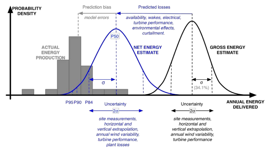
Fig. 7 Annual energy production distributions. Reprinted with permission from the National Renewable Energy Laboratory. [CSF16]

Besides energy yield, the process also predicts mean and extreme wind conditions that are relevant for wind turbine design, i.e. to guarantee that siting conditions meet the requirements to ensure the structural integrity of the wind turbines as per the IEC 61400-1 [ITC8819a] and IEC61400-3 [ITC8819b] (fixed offshore) standards.

The IEC 61400-15 working group has recently defined a framework for a standardized reporting of the wind resource, energy yield and turbine suitability process:

• The IEC 61400-15-1 complements IEC 61400-1 and 61400-3 in the reporting of site specific wind conditions and related atmospheric variables.

• The IEC 61400-15-2 addresses the asessment and reporting of wind resource and energy yield.

Whenever possible we shall use the definitions provided therein on relevant quantities of interest for flow model evaluation. The variables are integrated with a wind speed distribution that is representative of the design lifetime and they are defined at hub-height (\(z_{hub}\)) unless otherwise stated.

Note

As of June 2020, the IEC 61400-15 standards are in draft form.

Wind Resource

• Annual average wind speed at hub height (\(V_{ave}\)): wind speed averaged according to the definition of annual average, i.e. mean value of a set of measured data of sufficient size and duration to serve as an estimate of the expected value of the quantity. The averaging time interval shall be a whole number of years to average out non-stationary effects such as seasonality.

• Annual wind speed frequency distribution (\(f_{i,j}\)): Annual distribution of wind speeds as a function of wind direction i and/or wind speeds j. Wind speed is classified using 1 m/s bins and wind direction sectors are no wider than \(30^{\circ}\). Additional dimmensions related to turbulence characteristics like stability, turbulence intensity or wind shear could be used for additional granularity in the distribution.

• Weibull distribution: The probability distribution function used to describe the distribution of wind speeds over a period of one year, defined in terms of the scale parameter (\(C\)) and shape parameter \(k\).

  \[P_w(V) = 1 - exp\left[-(V/C)^k\right]\]

Energy Yield

• Gross annual energy production (\(AEP_{gross}\)): total amount of electrical energy produced by the Wind Turbine Generator System (WTGS), estimated by integrating the power curve with the wind speed frequency distribution and multiplying by the number of hours in a year. For a wind farm:

  \[AEP_{gross} = T\sum_{i,j,k} P_k(V_j) f_{i,j,k}\]

  where \(f_{i,j,k}\) is the annual wind speed frequency distribution at each turbine site k, \(P_k(V_j)\) is the power curve of each turbine at wind speed \(V_j\) and \(T\) = 8760 h is the number of hours in a year. The gross AEP is also defined as the AEP at a reference site, typically a meteorological mast, vertically extrapolated to hub-height and horizontally extrapolated to the turbine sites. This extrapolation is carried out by profile methods and flow models that predict speed-up effects due to terrain elevation and roughness changes, forest canopies and obstacles.

• (Net) Annual energy production (\(AEP\)): total amount of electrical energy delivered at the grid connection point after deducing all the energy losses that take place in the wind farm.

  \[AEP = AEP_{gross} - AEP_{gross}\prod_{l} \eta_{l}\]

  where \(\eta_{l}\) is the efficiency corresponding to the loss category l as per the IEC 61400-15, namely: electrical, availability, wake effect, curtailment, environmental and turbine performance. Each category includes a number of subcategories. For instance, wake losses are subdivided into internal (interarray effects), external (current farm-farm effects) and future (prospect farm-farm effects) wake losses. Internal wake losses are predicted by wake models to obtain the, so-called, array efficiency:

  \[\eta_{wake} = \frac{P_{wake}}{P_{gross}} = \frac{\sum_{i,j,k} Pw_k(V_j) f_{i,j,k}} {\sum_{i,j,k} P_k(V_j)f_{i,j,k}}\]

  where the efficiency is defined in terms of a power ratio with \(Pw_k\) being the power output predicted by the wake model at each turbine position k.

• Annual capacity factor (\(CF\)): the ratio between the AEP and the maximum possible annual energy output, an ideal case where all turbines would be producing at rated power throughout the year.

  \[CF = \frac{AEP}{T\sum_{k} Prated_k}\]

  where \(Prated_k\) is the rated power of each turbine. Alternatively, wind farm performance is defined in terms of the annual equivalent hours of the wind farm operating at rated power, i.e. \(AEH = CF \cdot T\)

The pre-construction energy yield assessment process will output a distribution of AEP defined in terms of the median \(P50\), where the actual AEP would be exceeded 50% of the time, and a standard deviation \(\sigma_{AEP}\) as a measure of the AEP uncertainty. Then, the prediction bias is the difference between the estimated P50 and the actual AEP

\[BIAS_{AEP} = AEP_{true} - AEP_{P50}\]

While each quantity of interest can be subject to uncertainty quantification individually, the main focus of the IEC 61400-15-2 standard is to predict the overall energy production uncertainty since this is directly connected to the financial performance of a wind project. This overall uncertainty is broken down into categories and subcategories by the standard to provide a common framework for the wind industry. Lee and Fields (2020) [LF20] provide a review of energy yield assessment prediction bias, losses and uncertainties following this framework. The review shows that while there has been a tendency towards the overestimation of P50, this has been progressively corrected and we are now approaching zero bias on average. The estimated mean AEP uncertainty remains at over 6% implying that there is room for improvement. Indeed, changing the uncertainty by 1% can lead to 3-5% change in the net present value of a wind farm [LF20].

Site Suitability

• Extreme wind speed with a recurrence interval of 50 years (\(V_{50}\)): Also called reference wind speed (\(V_{ref}\)) in the IEC 61400-1 standard to define WTGS classes. A turbine designed for a WTGS class with a reference wind speed \(V_{ref}\), is designed to withstand climates for which the extreme 10 min average wind speed with a recurrence period of 50 years at turbine hub-height is lower than or equal to \(V_{ref}\).

• Annual average flow inclination angle (\(\phi\)): The flow inclination is defined as the angle between a horizontal plane and the wind velocity vector at hub height:

  \[\phi = tan^{-1}\left(V_z/V_{xy}\right)\]

  where \(V_{xy}\) and \(V_{z}\) are the horizontal and vertical components of the wind speed. The flow inclination angle is positive if the wind velocity vector is pointing upwards. The annual average shall be taken as the energy weighted mean from all directions.

• Mean turbulence intensity (\(I\)): the ratio of the wind speed standard deviation to the mean wind speed determined from the same set of measured wind speed data and taken over a period of 10 minutes and a minimum sampling frequency of 5 seconds.

  \[I = \frac{\sigma_V}{V}\]

• Standard deviation of turbulence intensity (\(\sigma_{I}\)): The standard deviation of a sub set of the turbulence intensities (\(I\)). The sub set typically represents a bin within a wind speed- wind direction matrix.

• Average turbulence intensity at 15m/s (\(I_{15}\)): Mean turbulence intensity over all wind directions in 15m/s wind speed bin.

• Extreme ambient turbulence intensity: Extreme value of the ambient turbulence intensity with a return period of 50 years as a function of wind speed.

• Mean wind shear (\(\alpha\)): Wind shear, i.e. the variation of wind speed across a plane perpendicular to the wind direction, (or power law) exponent.

  \[V(z) = V(z_r)\left(\frac{z}{z_r}\right)^{\alpha}\]

Numerical Site Calibration

Todo

Define end-user requirements explicitely.

• Discuss IEC 61400-12-4 context

• Scope and Objectives

• Definitions of Quantities of Interest

• Impact of bias and uncertainty: set quality acceptance criteria

Multi-Scale Modeling of Wind Conditions

Sanz Rodrigo et al. (2016) [RAM+17] provide a review of mesoscale-to-microscale wind farm flow models of different fidelity levels considering meteorological and wind energy terminology. Each scale has different applications and quantities of interest, which will determine the orientation of the model evaluation strategy (Fig. 8).

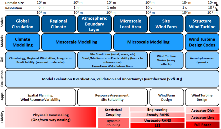
Fig. 8 Model-chain for wind farm flow modeling. © 2016 John Wiley & Sons, Ltd. Used with permission. [RAM+17]

Models can be coupled together to form a multi-scale modeling system where, for instance, the microscale sub-system (the wind farm) uses input data generated by the mesoscale sub-system to characterize the long-term wind climate distribution that modulates the local wind conditions. Similarly, an aerolastic model of the turbine sub-system can be used to predict detailed rotor aerodynamics responsible for wake generation in the wind farm wake model. A mind map elaborated during IEA-Task 31 Phase 3 shows the relationships between model building-blocks at different scales, input quantities and phenomena of interest for the intended use of these models (Fig. 9).

Fig. 9 Mind map of multi-scale models and phenomena of interest for wind conditions. Interactive mind map

The mind map breaks down the full complexity of atmospheric models into three scales:

1. Global: drives wind climate variability from seasons to decades at horizontal scales of tens of kilometers. Global reanalyses are typically used to characterize this variability and serve as input boundary condtions for mesoscale models.

2. Mesoscale: drives weather processes at regional level down to scales of the order of 1 km. Relevant mesoscale phenomena include: horizontal wind speed (gross AEP) gradients due large-scale topography, land-sea transitions and farm-farm (external wake) effect, low-level jets producing large wind shear during stable conditions, etc. Mesoscale models provide forcing for microscale models in the form of virtual masts, generalized wind climates, lateral boundary conditions or volumetric forzes (also called tendencies).

3. Microscale: drives turbulence and speed-up effects at site level at scales down to a few meters. Site effects depend on local changes in elevation and roughness, the presence of obstacles and forest canopies as well as thermal stratification across the atmospheric boundary-layer (ABL). Microscale effects are particularly important in complex terrain where relevant phenomena develop such as: flow separation and recirculation, gravity waves, gap flow, hydraulic jump, mountain-valley winds, etc. At microscale, wind farm wake models are embedded in atmospheric flow models to simulate internal wake effects that determine array efficiency.

Wake models are described in detail in the Multi-Scale Wind Farm Modeling section to simulate external and internal wake effects (array efficiency) and wind turbine loads.

Validation Strategy

Following the model evaluation process of Fig. 3, a validation strategy for wind conditions requires the provision of high-fidelity experiments targeting high-impact phenomena of interest, to validate the capacity of the flow model to deal with relevant physics, as well as long-term wind resource campaigns to demonstrate the added value that resolving these phenomena brings to the applications of interest. These applications typically involve integrating a discrete number of flow model simulations with a statistical methodology that provides the expected long-term mean or extreme values and the associated uncertainties. This should be done for a wide variety of wind climates and siting conditions to cover the widest operational range possible.

This validation strategy was implemented in the New European Wind Atlas (NEWA) project towards the development of a new methodology for the assessment of wind conditions that is based on a mesoscale to microscale model-chain approach [RAW+20]. The scope of the project was focused on wind conditions for wind resource and site assessment, i.e. without the influence of wind turbines. Therefore, the model-chain was devoted to atmospheric flow models with two applications in mind:

• Wind atlas for regional planning: the main focus was on the mesoscale model, to come up with a reference set-up of the Weather Research and Forecasting (WRF) model that could be used seamlessly across Europe. Through sensitivity analysis, the most suitable configuration was selected to produce a 30-year long simulation forced by ERA5 reanalysis data [HSW+20]. Then, this long-term wind climate was statistically downscaled to 50 m using the WAsP methodology. Hence, the wind atlas model-chain consists on physical downscaling down to 3 km resolution, to produce long-term time series of mesoscale wind characteristics, whose long-term wind climate distributions are then used as input data for a microscale model to produce high-resolution wind resource quantities. The validation strategy was based on a database of 291 meteorological masts, at least 40 m tall, made available by Vestas [DOW+20]. The main objective of the validation campaign was to determine the general quality of the wind atlas, categorized by regions and terrain complexity, determined by the ruggedness index RIX (Fig. 10) [MTL08]. A one year multi-physics ensemble run was also used to quantify the spread of mesoscale winds which would translate into input uncertainty for microscale models [RBH+19].

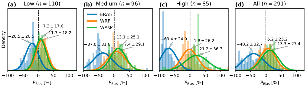
Fig. 10 Distributions of mean gross power bias, using the NREL 5MW reference turbine power curve, for the various stages of the NEWA model chain grouped by ruggedness index (RIX) category: low (a), medium (b), high (c), and all of the samples combined (d). © Author(s) 2020. CC BY 4.0 License. Used with permission. [DOW+20]

• Site assessment: here the main focus was on the microscale model, in particular, in the implementation of mesoscale forcing and boundary conditions for heterogeneous topography (complex terrain and forest canopies) using both Reynolds-Averaged Navier Stokes (RANS) and Large-Eddy Simulation (LES) turbulence models. Hence, the validation strategy seeked validation cases from detailed experiments where these modeling feutures would be tested in the prediction of mean flow and turbulence quantities. The range of experiments carried out in the NEWA allows testing over a wide range of siting conditions from offshore to coastal transitions to smooth and complex terrain with a without forest canopies. Next section provides an overview of these experiments and other open-access datasets that can be used to validate flow models.

Experiments and other Observational Datasets

The building-block validation hierarchy of Fig. 11 provides a framework to map validation datasets with phenomena of interest at different scales and show how they complement each other to cover a reasonably wide range of wind conditions. Site effects are modulated by the regional wind climate which is driven by synoptic weather and local mesoscale processes.

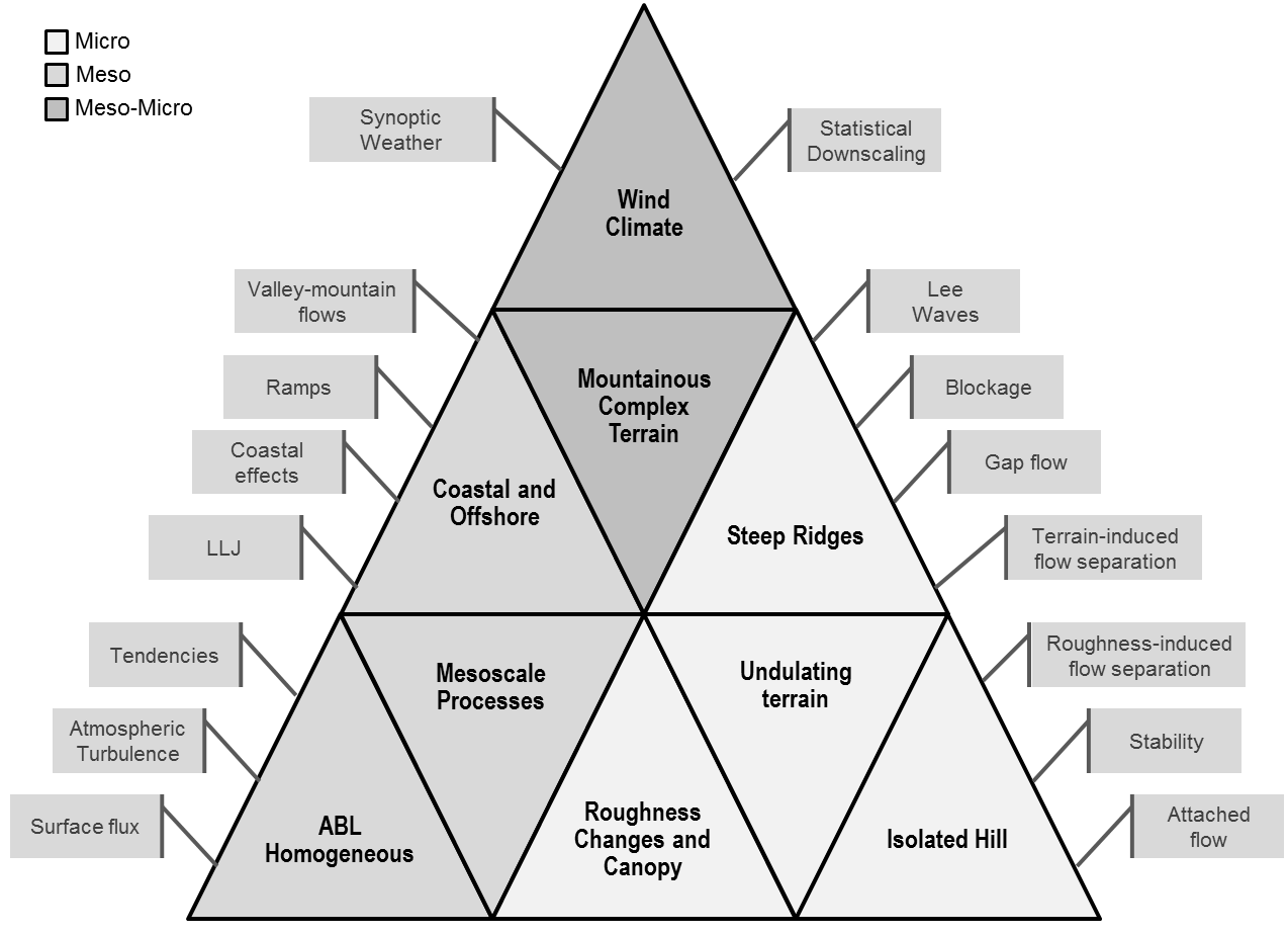
Fig. 11 Building-block validation hierarchy and phenomena of interest for wind conditions.

While long-term statistics of wind conditions are traditionally characterized with meteorological masts, many recent experiments include an intense operational period (IOP) of several weeks to months with extensive use of remote sensing equipment. In particular, scanning lidar systems allow to characterize the spatio-temporal structure of the flow field along scanning trajectories following a particular transect, or slicing vertical or horizontal planes ([MAA+17]). Table 2 provides a summary of experiments and other sources of open-access data for the validation of atmospheric flow models.

Table 2 Summary of open-access datasets for the validation of flow models for wind conditions

Dataset	Location	Period	Site Conditions	Key References & Repositories
Homogeneous ABL
Cabauw	This 200-m tall mast has been a reference in ABL research for its horizontally homogeneous conditions. The GABLS3 flow case is a diurnal cycle developing a strong nocturnal low-level [BBvM+14].
	Netherlands	Since 2008	Flat terrain	Cesar Database
Coastal and Offshore
Fino 1,2,3	Three 100-m tall offshore research platforms measuring boundary layer measurements between 30 and 100 m.
	North and Baltic Seas	Since 2003	Offshore	FINO1,2,3, BSH Database
Satellite SAR	Satellite SAR wind data archive from 2002
	Global	Since 2002	Offshore	DTU Satellite Winds [HHA+20]
RUNE	Near-shore wind resource from 8 lidars, one ocean buoy and satelite data
	Denmark	2015-11 to 2016-02	Near-shore	[FPL+16]
Ferry Lidar	Offshore wind resource from a ferry-mounted profiling lidar (65-275 m) along the South Baltic Sea from Kiel (Germany) to Klaipeda (Lithuania).
	Baltic Sea	2017-02 to 2017-06	Offshore	[GCDW18]
Roughness Changes and Forest Canopies
Ryningsnäs	200-m tall mast in a patchy forested site in simple terrain conditions
	Sweden	2011-10 to 2012-06	Forested simple terrain	[ASDB15], [AOEI19]
Østerild Balconies	Two horizontally scanning Doppler lidars, mounted on 250-m high masts and measuring at 50 and 200 m the flow above patchy forest
	Denmark	2016-04 to 2016-08	Forested flat terrain	[KMDV18]
Isolated Hill
Askervein	116 m high smooth hill isolated in all wind directions but the NE-E sector. Over 50 masts installed, 35 of them of 10 m height installed along transects following the main axes of the hill
	Scotland	1982/1983	Smooth hill	[TT87], [TT83] [TT85]
Rödeser Berg (Kassel)	200-m tall forested hill equipped with a 200-m mast at the hill top, a 140-m mast at the inflow and scanning Doppler lidars mapping a transect along the prevailing wind direction
	Germany	2016-10 to 2017-01	Forested hill	[DWG19]
Undulating Terrain
Hornamossen	10-km long transect consisting of 9 remote sensing profilers and one 180-m flux-profile mast in forested and moderately complex terrain. Surface pressure gradient measurements
	Sweden	2015-06 to 2017-07	Forested rolling hills	[MAA+17]
Steep Ridges
Bolund	12-m high hill surrounded by water in all directions except to the E. An almost vertical escarpment faces the prevailing W-SW sector. 10 masts equiped with sonic and cup anemometers.
	Denmark	2007-2008	Small isolated ridge	[BBC+09], [BMB+11], [BSB+11]
Perdigão	50 masts, 20 scanning lidars, 7 profiling lidars and other meteorological equipment distributed along and across two parallel steep ridges.
	Portugal	2016-12 to 2017-06	Double ridge	FEUP-Porto Database, NCAR Database, [FMP+19]
Mountaineous Complex Terrain
Alaiz (ALEX17)	5 scanning Doppler lidars measuring a Z-shaped 10-km long transect along the ridge tops and across the valley together with a windRASS profiler, 7 tall masts and 10 surface stations
	Spain	2017-07 to 2019-07	Ridge-valley-mountain	[CBGSR+19], [SMV+19], [SMV+20]

Note

Other open-access datasets can be added when they have been used for flow model validation (provide references)

Phenomena of Interest

Todo

Most recent PIRT addressing relevent phenomena for wind conditions.

• List of physical phenomena providing definitions and references

• PIRT table from MMC

Benchmarks on Flow Phenomena

Following the building-block approach illustrated in Fig. 11, we provide a comprehensive list of benchmarks for the design and testing of atmospheric flow models. These test cases are derived from theory and high-fidelity experiments to target specific flow phenomena that is considered relevant for the intended uses of the models. From Monin-Obukhov theory in homogeneous conditions to flow over complex terrain and forest canopies, a hierarchy of flow cases is provided in each building-block.

The Homogeneous Atmospheric Boundary Layer (ABL)

The ABL building-block of Fig. 12 deals with the horizontally homogeneous atmospheric boundary-layer. A hierarchy of verification and validation cases is suggested to progressively incorporate essential physics, namely:

1. Monin-Obukhov similarity theory (MOST) for surface-layer steady-state conditions depending on roughness and stability [MO54].

2. Leipzig ABL wind profile in neutral steady-state conditions [Let50].

3. GABLS1 stable ABL under uniform geostrophic wind and surface cooling [CHB+06].

4. GABLS2 diurnal cycle under uniform geostrophic wind and varying surface temperature [KSH+10].

5. GABLS3 diurnal cycle under realistic mesoscale forcing and varying surface boundary conditions [BBvM+14].

6. Cabauw annual integration of the wind climate to predict quantities of interest for the intended use wind resource assessment and turbine siting [RAG+18] (see Assessment of Wind Resource, Energy Yield and Site Suitability section).

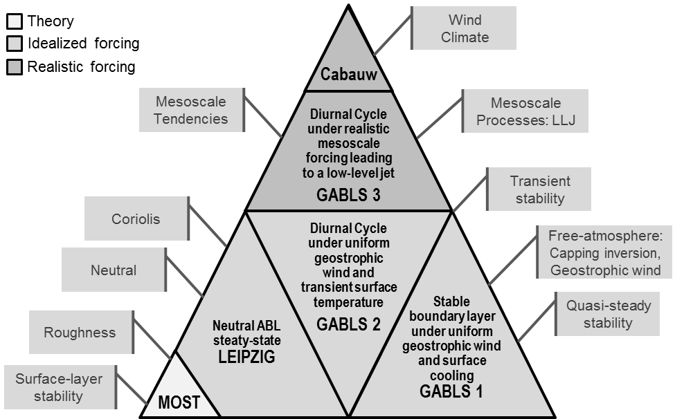
Fig. 12 V&V hierarchy for the ABL building-block.

Benchmarks for MOST and Leipzig were conducted during Wakebench Phase 1 [RGA+14]. The GEWEX Atmospheric Boundary Layer Studies (GABLS), developed by the boundary-layer meteorology community [HSB+13], can be adopted by the wind energy community by focusing the evaluation on rotor-based quantities of interest [SRCK17]. The GABLS3 and Cabauw benchmarks were conducted in Wakebench Phase 2 [RAA+17][RAG+18].

• Monin Obukhov Similarity Theory (MOST)
• Leipzig Neutral ABL Profile (Leipzig)
• Diurnal Cycle Leading to a Nocturnal Low-Level Jet (GABLS3)

Coastal-Offshore

The marine atmospheric boundary layer is formed through exchanges of momentum moisture and heat across the air-sea interface. Fig. 21 shows a schematic of the physical processes that take place in the coupled atmospheric-ocean boundary layer [ECC+07]. Mesoscale variability and wave-induced effects produce deviations from land-based turbulence spectra and flux-profile relationships used in ABL parameterizations [SHB+99]. The coastal region, where most offshore wind energy is deployed, is subject to large mesoscale variability influenced by coastal topography and temperature gradients between land and sea [DOMS15]. These heterogeneous conditions generate important horizontal wind speed gradients breaking MOST assumptions on which many wake models are based. Furthermore, frequent stable conditions develop due to large land-see temperature contrast producing large-shear low-level jets (LLJ) in shallow boundary-layers and gravity waves that increase wind farm global blockage [AM18]. In extreme wind conditions, wave-induced shear-stress becomes dominant favouring the use of a wind-wave coupled model [LDB+19].

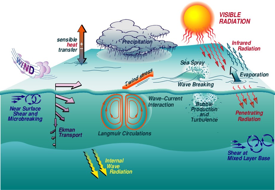
Fig. 21 Air-sea interaction processes in the marine boundary layer. © American Meteorological Society. Used with permission. [ECC+07]

The NEWA project has produced two benchmarks suitable for the assessment of the coastal-offshore boundary layer. The Ferry-Lidar experiment consist on following a ferry-mounted profiling lidar, for a period of 4 months, along a regular route in the Southern Baltic Sea between Kiel (Germany) and Klaipeda (Lithuania). The RUNE experiment comprises measurements from 8 lidars and a buoy to measure the evolution of the wind speed along a ~8 km fetch.

• The Ferry-Lidar Marine Boundary-Layer (Ferry-Lidar)

Todo

• Complete Ferry-Lidar benchmark.

• Add RUNE benchmark.

Forest Canopy

A canopy is considered when the roughness elements over the ground surface are of significant size compared to the height of interest (e.g. hub-height). Here we shall focus on forest canopies although the term could be also applied for a urban canopy or a wind farm canopy. The classical interpretation of the flow over a forest canopy is that of a displaced logarithmic profile originating by the momentum absortion through aerodynamic drag across the depth of the canopy [JCJJ94], where the displacement height depends on the distribution of the drag through the foliage. Within the canopy the flow is highly turbulent and heterogeneous which prevents us from extending MOST to the canopy layer as if it was a rough lower boundary. A more realistic approach requires to model explicitely the distribution of drag and the energy balance between the surface and the air aloft to characterize the flow above and within the canopy.

The structure of the turbulent flow in horizontally homogeneous canopies have been the object of study of numerous experiments ranging from wind tunnel models (e.g. [BFR94]) to tall forests [JCJJ94]. All the profiles display a characteristic inflexion point near the canopy top which separates the canopy flow from the boundary layer profile above. A constant shear stress region is present in the free-stream which decreases rapidly as momentum is absorbed by the canopy.

Heterogeneous forest canopies combine patches of trees of different heights and foliage density that typically change throughout the year. Aerial lidar scans are used to map the tree height and plant area density [BBT+15]. Highly heterogeneous conditions happen at forest edges as the flow transitions through an internal boundary layer towards a developed canopy boundary layer [DBM14] [BDBD17].

The Ryningsnäs experiment was used in the NEWA project to validate ABL models in neutral conditions [IAA+18] considering mean vertical profiles of wind speed and turbulence intensity for different wind direction sectors. A follow-up experiment, Hornamossen, studied the mean flow along a transect of 9 remote sensing profilers and a reference 180-m met mast over undulated forested terrain [MAA+17]. The Østerild Balconies experiment deployed two horizontally scanning lidars on vertical masts at 50 and 200 m to characterize the heteorogeneous mean flow above the canopy over a relatively flat and semi-forested terrain [KMDV18].

• The Ryningsnäs Forest Canopy ABL (Ryningsnäs)
• The Hornamossen Diurnal-Cycle in Forested Undulating Terrain (Hornamossen)

Todo

• Complete Ryningsnas and Hornamossen benchmarks.

Isolated Hills

To study the influence of terrain elevation changes on the ABL we first study the flow over isolated hills, i.e. when the inflow conditions are relatively homogeneous and the height of the hill is small compared to the ABL height (~100 m, where surface-layer turbulence dominates the flow). These conditions have been traditionally used to validate linearized flow models since pioneering work from Jackson and Hunt (1975) [JH75] that led to the Askervein experiment in 1982 and 1983 [TT87]. This is a 116-m high hill in Scothland with gentle slopes (i.e. less than ~30% to prevent flow separation) and homogeneous inflow from the SW, where a quasi-steady flow case in neutral conditions was generated. This case became a golden benchmark to test flow-over-hill models until the Bolund hill experiment in 2007 [BBC+09] [BMB+11]: a 12-m high isolated ridge with steep terrain in the prevailing wind direction, suitable for testing non-linear flow models still in surface-layer and predominanantly neutral conditions [BSB+11].

The idealized inflow conditions assumed in flow-over-hill studies are suitable for wind tunnel experiments. These are adequate for parametric testing of the flow under different hill shapes, surface roughnesses and stability coditions, e.g. [FRBA90], [KP00], [RAV+04], [RV05], [WPA11].

The NEWA experiment at the Röderser Berg hill near Kassel is the most recent field campaign in the isolated hills category in the wind energy context. This ~200 m hill, covered by a forest of 20-30 m tree-heights, includes two 200-m tall masts at the inflow and hilltop and doppler-lidar longitudinal profiles across the hill to measure the speed-up at two heights (80 and 135 m) [DWG19].

• The Askervein Isolated Smooth Hill (Askervein)
• The Bolund Isolated Steep Hill (Bolund)
• The Rödeser Berg Forested Smooth Hill (Rödeser Berg)

Todo

• Complete Rodeser Berg benchmark.

Complex Terrain

According to the IEC 61400-12-1 standard [ITC8817], in the context of power performance testing, complex terrain is terrain surrounding the test site that features significant variations in topography and terrain obstacles that may cause flow distortion, i.e. significant variations in the wind conditions that affect turbine performance (wind shear, turbulence intensity, etc). To categorize terrain complexity, three types of complex terrain are defined [ITC8817]:

• Type A: does not have significant changes in elevation relative to the hub height or particularly steep slopes over long distances. Examples of Type A terrain include gentle rolling hills, and turbine located on a ridge facing a plane.

• Type B: includes mountains, ridgelines, large hills and hilly sites with moderate to steepy sloping terrain and significant changes in elevation relative to the hub height.

• Type C: typically have a steep terrain feature such as a mountain or canyon that may cause flow separation directly upwind of the site of interest. These conditions create drastic changes in wind conditions

These definitions are relative to the terrain conditions seen at a target wind turbine site and, therefore, depend on the wind direction sector under consideration.

Terrain complexity has been quantified using the ruggedness index RIX which measures the fraction of terrain surface that is steeper than a critical slope of 30-40%. This index is related to the likelihood of flow separation, an important factor in the performance of flow models [MTL08]. In effect, the difference between the RIX at the reference (measured) site and that at the predicted site, \(\Delta RIX\) shows positive correlation with the prediction error of a linearized model when the flow is dominated by terrain effects, i.e. without much influence from thermal effects, drastic roughness changes, forest canopy effects or mesoscale effects [MTL08].

Fig. 21 shows a schematic of the Perdigão double-hill experiment illustrating the most relevant physical phenomena [FMP+19]. While the flow near the surface is dominated by terrain effects, wind conditions at turbine-relevant heights are modulated by mesoscale thermal and (synoptic) topographic forcings. Thermal circulation effects due to differences in temperature between the hilltop and the valley cause upslope (anabatic) and katabatic (downslope) winds driven by buoyancy forces. Under synoptic conditions the flow is determined by atmospheric stability. In stable conditions, turbulence mixing is reduced mitigating flow separation but favouring the generation of multiple flow phenomena: lee waves, hydraulic jumps, shear layers, upstream blocking, etc. In neutral and unstable conditions terrain-induced flow separation is more likely producing recirculation in the lee side and other unsteady phenomena due to the interaction with downstream topography.

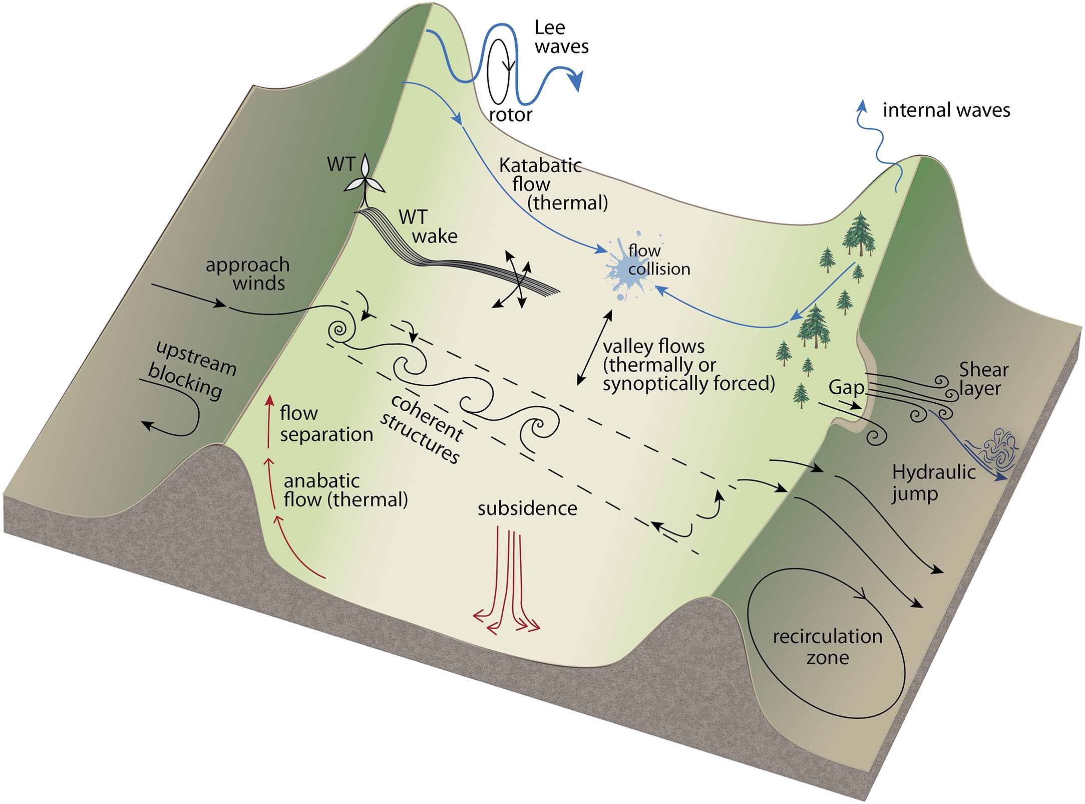
Fig. 26 Phenomena of interest in the Perdigão experiment. ©American Meteorological Society. Used with permission. [FMP+19]

Besides Perdigão, the NEWA project produced a follow-up experiment in complex terrain at the Alaiz site [SMV+20] to study the interaction between the Tajonar ridge, of similar height as Perdigão hills (~250 m), and the Alaiz mountain range (~700 m), both separated by a ~ 6-km wide valley. The high altitude of Alaiz results in larger interaction with the ABL structure and mesoscale flow.

Todo

• Perdigão benchmark.

• Alaiz diurnal cycles benchmark.

Benchmarks on Intended Use

This section describes benchmarks in the application space, where flow models are integrated with the statistics of the long-term wind climate to predict the quantities of interest that are relevant for the inteded uses of the model (see Intended Use section). Before running these benchmarks, flow models should have demonstrated their predictive capacity by validating as many flow cases as possible from the Benchmarks on Flow Phenomena section. This way, it will be easier to understand the limitations of the model and relate them to the resulting prediction bias. In other words, the objective is to quantify the impact that the formal V&V process has on the applications of interest and highlight gaps that should be addressed in the next round of targeted experiments and validation campaigns.

The assessment shall be done on as many sites as possible to cover a wide range of operational conditions. This will require the provision of measurement campaigns from industry to complement the publicly available experimental campaigns.

Assessment of Wind Resource, Energy Yield and Site Suitability

The NEWA project offers a number of public long-term measurement campaigns that can be used to validate AEP and long-term wind conditions in different European wind climates and topographic conditions. A baseline case in horizontally homogeneous conditions is based at the Cabauw Experimental Site for Atmospheric Research (CESAR) in the Netherlands.

• Annual Energy Yield Assessment and Wind Conditions at Cabauw (Cabauw)

Todo

• Add Rödeser Berg AEP benchmark

Numerical Site Calibration

Todo

• Add Alaiz site calibration.

References

AM18

Dries Allaerts and Johan Meyers. Gravity Waves and Wind-Farm Efficiency in Neutral and Stable Conditions. Boundary-Layer Meteorol, 166(2):269–299, February 2018. URL: https://doi.org/10.1007/s10546-017-0307-5 (visited on 2020-10-22), doi:10.1007/s10546-017-0307-5.

AOEI19

Johan Arnqvist, H. Olivares-Espinosa, and S. Ivanell. Investigation of Turbulence Accuracy When Modeling Wind in Realistic Forests Using LES. In Ramis Örlü, Alessandro Talamelli, Joachim Peinke, and Martin Oberlack, editors, Progress in Turbulence VIII, Springer Proceedings in Physics, 291–296. Cham, 2019. Springer International Publishing. doi:10.1007/978-3-030-22196-6_46.

ASDB15

Johan Arnqvist, Antonio Segalini, Ebba Dellwik, and Hans Bergström. Wind Statistics from a Forested Landscape. Boundary-Layer Meteorol, 156(1):53–71, July 2015. URL: https://doi.org/10.1007/s10546-015-0016-x (visited on 2020-07-22), doi:10.1007/s10546-015-0016-x.

BSB+11(1,2)

A. Bechmann, N. N. Sørensen, J. Berg, J. Mann, and P.-E. Réthoré. The Bolund Experiment, Part II: Blind Comparison of Microscale Flow Models. Boundary-Layer Meteorol, 141(2):245, August 2011. URL: https://doi.org/10.1007/s10546-011-9637-x (visited on 2020-07-23), doi:10.1007/s10546-011-9637-x.

BBC+09(1,2)

Andreas Bechmann, Jacob Berg, Michael Courtney, Hans Ejsing Jørgensen, Jakob Mann, and Niels N. Sørensen. The Bolund Experiment: Overview and Background. Technical Report, Danmarks Tekniske Universitet, 2009. URL: https://orbit.dtu.dk/en/publications/the-bolund-experiment-overview-and-background (visited on 2020-07-23).

BMB+11(1,2)

J. Berg, J. Mann, A. Bechmann, M. S. Courtney, and H. E. Jørgensen. The Bolund Experiment, Part I: Flow Over a Steep, Three-Dimensional Hill. Boundary-Layer Meteorol, 141(2):219, July 2011. URL: https://doi.org/10.1007/s10546-011-9636-y (visited on 2020-07-23), doi:10.1007/s10546-011-9636-y.

BBvM+14(1,2)

Fred C. Bosveld, Peter Baas, Erik van Meijgaard, Evert I. F. de Bruijn, Gert-Jan Steeneveld, and Albert A. M. Holtslag. The Third GABLS Intercomparison Case for Evaluation Studies of Boundary-Layer Models. Part A: Case Selection and Set-Up. Boundary-Layer Meteorol, 152(2):133–156, August 2014. URL: https://doi.org/10.1007/s10546-014-9917-3 (visited on 2020-10-06), doi:10.1007/s10546-014-9917-3.

BBT+15

Louis-Étienne Boudreault, Andreas Bechmann, Lasse Tarvainen, Leif Klemedtsson, Iurii Shendryk, and Ebba Dellwik. A LiDAR method of canopy structure retrieval for wind modeling of heterogeneous forests. Agricultural and Forest Meteorology, 201:86–97, February 2015. URL: http://www.sciencedirect.com/science/article/pii/S0168192314002652 (visited on 2020-10-23), doi:10.1016/j.agrformet.2014.10.014.

BDBD17

Louis-Étienne Boudreault, Sylvain Dupont, Andreas Bechmann, and Ebba Dellwik. How Forest Inhomogeneities Affect the Edge Flow. Boundary-Layer Meteorol, 162(3):375–400, March 2017. URL: https://doi.org/10.1007/s10546-016-0202-5 (visited on 2020-10-23), doi:10.1007/s10546-016-0202-5.

BFR94

Y. Brunet, J. J. Finnigan, and M. R. Raupach. A wind tunnel study of air flow in waving wheat: Single-point velocity statistics. Boundary-Layer Meteorol, 70(1):95–132, July 1994. URL: https://doi.org/10.1007/BF00712525 (visited on 2020-10-23), doi:10.1007/BF00712525.

CBGSR+19

Elena Cantero, Fernando Borbón Guillén, Javier Sanz Rodrigo, Pedro Santos, Jakob Mann, Nikola Vasiljević, Michael Courtney, Daniel Martínez Villagrasa, Belén Martí, and Joan Cuxart. Alaiz Experiment (ALEX17): Campaign and Data Report. Technical Report, Zenodo, May 2019. Publisher: Zenodo. URL: https://zenodo.org/record/3187482 (visited on 2020-07-22), doi:10.5281/zenodo.3187482.

CSF16(1,2)

Andrew Clifton, Aaron Smith, and Michael Fields. Wind Plant Preconstruction Energy Estimates. Current Practice and Opportunities. Technical Report NREL/TP-5000-64735, National Renewable Energy Lab. (NREL), Golden, CO (United States), April 2016. URL: https://www.osti.gov/biblio/1248798 (visited on 2020-11-03), doi:10.2172/1248798.

CHB+06

J. Cuxart, A. A. M. Holtslag, R. J. Beare, E. Bazile, A. Beljaars, A. Cheng, L. Conangla, M. Ek, F. Freedman, R. Hamdi, A. Kerstein, H. Kitagawa, G. Lenderink, D. Lewellen, J. Mailhot, T. Mauritsen, V. Perov, G. Schayes, G-J. Steeneveld, G. Svensson, P. Taylor, W. Weng, S. Wunsch, and K-M. Xu. Single-Column Model Intercomparison for a Stably Stratified Atmospheric Boundary Layer. Boundary-Layer Meteorol, 118(2):273–303, February 2006. URL: https://doi.org/10.1007/s10546-005-3780-1 (visited on 2020-10-06), doi:10.1007/s10546-005-3780-1.

DBM14

Ebba Dellwik, Ferhat Bingöl, and Jakob Mann. Flow distortion at a dense forest edge. Quarterly Journal of the Royal Meteorological Society, 140(679):676–686, 2014. _eprint: https://rmets.onlinelibrary.wiley.com/doi/pdf/10.1002/qj.2155. URL: https://rmets.onlinelibrary.wiley.com/doi/abs/10.1002/qj.2155 (visited on 2020-10-23), doi:10.1002/qj.2155.

DOW+20(1,2)

Martin Dörenkämper, Bjarke T. Olsen, Björn Witha, Andrea N. Hahmann, Neil N. Davis, Jordi Barcons, Yasemin Ezber, Elena García-Bustamante, J. Fidel González-Rouco, Jorge Navarro, Mariano Sastre-Marugán, Tija Sīle, Wilke Trei, Mark Žagar, Jake Badger, Julia Gottschall, Javier Sanz Rodrigo, and Jakob Mann. The Making of the New European Wind Atlas – Part 2: Production and evaluation. Geoscientific Model Development, 13(10):5079–5102, October 2020. Publisher: Copernicus GmbH. URL: https://gmd.copernicus.org/articles/13/5079/2020/ (visited on 2020-10-27), doi:https://doi.org/10.5194/gmd-13-5079-2020.

DOMS15

Martin Dörenkämper, Michael Optis, Adam Monahan, and Gerald Steinfeld. On the Offshore Advection of Boundary-Layer Structures and the Influence on Offshore Wind Conditions. Boundary-Layer Meteorol, 155(3):459–482, June 2015. URL: https://doi.org/10.1007/s10546-015-0008-x (visited on 2020-10-22), doi:10.1007/s10546-015-0008-x.

DWG19(1,2)

Martin Dörenkämper, Björn Witha, and Julia Gottschall. Large-Eddy and Reynolds-Averaged-Navier Stokes simulations of the Kassel forested hill - Rödeser Berg (Deliverable D2.13). Technical Report, Zenodo, October 2019. Publisher: Zenodo. URL: https://zenodo.org/record/3519169 (visited on 2020-07-22), doi:10.5281/zenodo.3519169.

ECC+07(1,2)

James Edson, Timothy Crawford, Jerry Crescenti, Tom Farrar, Nelson Frew, Greg Gerbi, Costas Helmis, Tihomir Hristov, Djamal Khelif, Andrew Jessup, Haf Jonsson, Ming Li, Larry Mahrt, Wade McGillis, Albert Plueddemann, Lian Shen, Eric Skyllingstad, Tim Stanton, Peter Sullivan, Jielun Sun, John Trowbridge, Dean Vickers, Shouping Wang, Qing Wang, Robert Weller, John Wilkin, Albert J. Williams, D. K. P. Yue, and Chris Zappa. The Coupled Boundary Layers and Air–Sea Transfer Experiment in Low Winds. Bull. Amer. Meteor. Soc., 88(3):341–356, March 2007. Publisher: American Meteorological Society. URL: https://journals.ametsoc.org/bams/article/88/3/341/59046/The-Coupled-Boundary-Layers-and-Air-Sea-Transfer (visited on 2020-10-22), doi:10.1175/BAMS-88-3-341.

FMP+19(1,2,3)

H. J. S. Fernando, J. Mann, J. M. L. M. Palma, J. K. Lundquist, R. J. Barthelmie, M. Belo-Pereira, W. O. J. Brown, F. K. Chow, T. Gerz, C. M. Hocut, P. M. Klein, L. S. Leo, J. C. Matos, S. P. Oncley, S. C. Pryor, L. Bariteau, T. M. Bell, N. Bodini, M. B. Carney, M. S. Courtney, E. D. Creegan, R. Dimitrova, S. Gomes, M. Hagen, J. O. Hyde, S. Kigle, R. Krishnamurthy, J. C. Lopes, L. Mazzaro, J. M. T. Neher, R. Menke, P. Murphy, L. Oswald, S. Otarola-Bustos, A. K. Pattantyus, C. Veiga Rodrigues, A. Schady, N. Sirin, S. Spuler, E. Svensson, J. Tomaszewski, D. D. Turner, L. van Veen, N. Vasiljević, D. Vassallo, S. Voss, N. Wildmann, and Y. Wang. The Perdigão: Peering into Microscale Details of Mountain Winds. Bull. Amer. Meteor. Soc., 100(5):799–819, May 2019. Publisher: American Meteorological Society. URL: https://journals.ametsoc.org/bams/article/100/5/799/344800/The-Perdigao-Peering-into-Microscale-Details-of (visited on 2020-07-22), doi:10.1175/BAMS-D-17-0227.1.

FRBA90

J. J. Finnigan, M. R. Raupach, E. F. Bradley, and G. K. Aldis. A wind tunnel study of turbulent flow over a two-dimensional ridge. Boundary-Layer Meteorol, 50(1):277–317, March 1990. URL: https://doi.org/10.1007/BF00120527 (visited on 2020-10-26), doi:10.1007/BF00120527.

FPL+16

Rogier Floors, Alfredo Peña, Guillaume Lea, Nikola Vasiljević, Elliot Simon, and Michael Courtney. The RUNE Experiment—A Database of Remote-Sensing Observations of Near-Shore Winds. Remote Sensing, 8(11):884, November 2016. Number: 11 Publisher: Multidisciplinary Digital Publishing Institute. URL: https://www.mdpi.com/2072-4292/8/11/884 (visited on 2020-07-22), doi:10.3390/rs8110884.

GCDW18

Julia Gottschall, Eleonora Catalano, Martin Dörenkämper, and Björn Witha. The NEWA Ferry Lidar Experiment: Measuring Mesoscale Winds in the Southern Baltic Sea. Remote Sensing, 10(10):1620, October 2018. Number: 10 Publisher: Multidisciplinary Digital Publishing Institute. URL: https://www.mdpi.com/2072-4292/10/10/1620 (visited on 2020-07-22), doi:10.3390/rs10101620.

HSW+20

Andrea N. Hahmann, Tija Sile, Björn Witha, Neil N. Davis, Martin Dörenkämper, Yasemin Ezber, Elena García-Bustamante, J. Fidel González Rouco, Jorge Navarro, Bjarke T. Olsen, and Stefan Söderberg. The Making of the New European Wind Atlas, Part 1: Model Sensitivity. Geoscientific Model Development Discussions, pages 1–33, March 2020. Publisher: Copernicus GmbH. URL: https://gmd.copernicus.org/preprints/gmd-2019-349/ (visited on 2020-07-22), doi:https://doi.org/10.5194/gmd-2019-349.

HHA+20

Charlotte B. Hasager, Andrea N. Hahmann, Tobias Ahsbahs, Ioanna Karagali, Tija Sile, Merete Badger, and Jakob Mann. Europe’s offshore winds assessed with synthetic aperture radar, ASCAT and WRF. Wind Energy Science, 5(1):375–390, March 2020. Publisher: Copernicus GmbH. URL: https://wes.copernicus.org/articles/5/375/2020/ (visited on 2020-07-22), doi:https://doi.org/10.5194/wes-5-375-2020.

HSB+13

A. a. M. Holtslag, G. Svensson, P. Baas, S. Basu, B. Beare, A. C. M. Beljaars, F. C. Bosveld, J. Cuxart, J. Lindvall, G. J. Steeneveld, M. Tjernström, and B. J. H. Van De Wiel. Stable Atmospheric Boundary Layers and Diurnal Cycles: Challenges for Weather and Climate Models. Bull. Amer. Meteor. Soc., 94(11):1691–1706, November 2013. Publisher: American Meteorological Society. URL: https://journals.ametsoc.org/bams/article/94/11/1691/60301/Stable-Atmospheric-Boundary-Layers-and-Diurnal (visited on 2020-10-14), doi:10.1175/BAMS-D-11-00187.1.

ITC8817(1,2)

IEC-TC88. IEC 61400-12-1 Wind turbines - Part 12:1: Power performance measurements of electricity producing wind turbines. Standard IEC 61400-12-1:2017 ed. 2.0, International Electrotechnical Commission, Geneva, CH, September 2017. URL: https://webstore.iec.ch/publication/26603 (visited on 2020-10-27).

ITC8819a

IEC-TC88. IEC 61400-1 Wind energy generation systems - Part 1: Design requirements. Standard IEC 61400-1:2019 ed. 4.0, International Electrotechnical Commission, Geneva, CH, February 2019. URL: https://webstore.iec.ch/publication/26423 (visited on 2020-11-03).

ITC8819b

IEC-TC88. IEC 61400-3-1 Wind energy generation systems - Part 3-1: Design requirements for fixed offshore wind turbines. Standard IEC 61400-3-1:2019 ed. 1.0, International Electrotechnical Commission, Geneva, CH, April 2019. URL: https://webstore.iec.ch/publication/29360 (visited on 2020-11-03).

IAA+18

Stefan Ivanell, Johan Arnqvist, Matias Avila, Dalibor Cavar, Roberto Aurelio Chavez-Arroyo, Hugo Olivares-Espinosa, Carlos Peralta, Jamal Adib, and Björn Witha. Micro-scale model comparison (benchmark) at the moderately complex forested site Ryningsnäs. Wind Energy Science, 3(2):929–946, December 2018. Publisher: Copernicus GmbH. URL: https://wes.copernicus.org/articles/3/929/2018/ (visited on 2020-10-23), doi:https://doi.org/10.5194/wes-3-929-2018.

JCJJ94(1,2)

Kaimal J.C. and Finnigan J.J. Atmospheric Boundary Layer Flows. Their Structure and Measurement. Oxford University Press, New York, 1994. ISBN 0-19-506239-6.

JH75

P. S. Jackson and J. C. R. Hunt. Turbulent wind flow over a low hill. Quarterly Journal of the Royal Meteorological Society, 101(430):929–955, 1975. _eprint: https://rmets.onlinelibrary.wiley.com/doi/pdf/10.1002/qj.49710143015. URL: https://rmets.onlinelibrary.wiley.com/doi/abs/10.1002/qj.49710143015 (visited on 2020-10-26), doi:10.1002/qj.49710143015.

KMDV18(1,2)

Ioanna Karagali, Jakob Mann, Ebba Dellwik, and Nikola Vasiljević. New European Wind Atlas: The østerild balconies experiment. J. Phys.: Conf. Ser., 1037:052029, June 2018. Publisher: IOP Publishing. URL: https://doi.org/10.1088%2F1742-6596%2F1037%2F5%2F052029 (visited on 2020-07-22), doi:10.1088/1742-6596/1037/5/052029.

KP00

H. G. Kim and V. C. Patel. Test Of Turbulence Models For Wind Flow Over Terrain With Separation And Recirculation. Boundary-Layer Meteorology, 94(1):5–21, January 2000. URL: https://doi.org/10.1023/A:1002450414410 (visited on 2020-07-23), doi:10.1023/A:1002450414410.

KSH+10

Vijayant Kumar, Gunilla Svensson, A. a. M. Holtslag, Charles Meneveau, and Marc B. Parlange. Impact of Surface Flux Formulations and Geostrophic Forcing on Large-Eddy Simulations of Diurnal Atmospheric Boundary Layer Flow. J. Appl. Meteor. Climatol., 49(7):1496–1516, July 2010. Publisher: American Meteorological Society. URL: https://journals.ametsoc.org/jamc/article/49/7/1496/13293/Impact-of-Surface-Flux-Formulations-and (visited on 2020-10-06), doi:10.1175/2010JAMC2145.1.

LDB+19

Xiaoli Guo Larsén, Jianting Du, Rodolfo Bolaños, Marc Imberger, Mark C. Kelly, Merete Badger, and Søren Larsen. Estimation of offshore extreme wind from wind-wave coupled modeling. Wind Energy, 22(8):1043–1057, 2019. _eprint: https://onlinelibrary.wiley.com/doi/pdf/10.1002/we.2339. URL: https://onlinelibrary.wiley.com/doi/abs/10.1002/we.2339 (visited on 2020-10-22), doi:10.1002/we.2339.

LF20(1,2)

Joseph C. Y. Lee and M. Jason Fields. An Overview of Wind Energy Production Prediction Bias, Losses, and Uncertainties. Wind Energy Science Discussions, pages 1–82, July 2020. Publisher: Copernicus GmbH. URL: https://wes.copernicus.org/preprints/wes-2020-85/ (visited on 2020-07-22), doi:https://doi.org/10.5194/wes-2020-85.

Let50

Heinz Lettau. A Re-examination of the “Leipzig Wind Profile” Considering some Relations between Wind and Turbulence in the Frictional Layer. Tellus, 2(2):125–129, 1950. _eprint: https://onlinelibrary.wiley.com/doi/pdf/10.1111/j.2153-3490.1950.tb00321.x. URL: https://onlinelibrary.wiley.com/doi/abs/10.1111/j.2153-3490.1950.tb00321.x (visited on 2020-10-06), doi:10.1111/j.2153-3490.1950.tb00321.x.

M12

Brower M. Wind Resource Assessment: A Practical Guide to Developing a Wind Project \textbar Wiley. Wiley, 2012. ISBN 978-1-118-02232-0. URL: https://www.wiley.com/en-es/Wind+Resource+Assessment%3A+A+Practical+Guide+to+Developing+a+Wind+Project-p-9781118022320 (visited on 2020-11-03).

MAA+17(1,2,3)

J. Mann, N. Angelou, J. Arnqvist, D. Callies, E. Cantero, R. Chávez Arroyo, M. Courtney, J. Cuxart, E. Dellwik, J. Gottschall, S. Ivanell, P. Kühn, G. Lea, J. C. Matos, J. M. L. M. Palma, L. Pauscher, A. Peña, J. Sanz Rodrigo, S. Söderberg, N. Vasiljevic, and C. Veiga Rodrigues. Complex terrain experiments in the New European Wind Atlas. Philosophical Transactions of the Royal Society A: Mathematical, Physical and Engineering Sciences, 375(2091):20160101, April 2017. Publisher: Royal Society. URL: https://royalsocietypublishing.org/doi/full/10.1098/rsta.2016.0101 (visited on 2020-07-22), doi:10.1098/rsta.2016.0101.

MO54

A S Monin and A M Obukhov. Basic laws of turbulent mixing in the surface layer of the atmosphere. Contrib. Geophys. Inst. Acad. Sci. USSR, pages 163–187, 1954.

MTL08(1,2,3)

Niels Gylling Mortensen, Andrew Tindal, and Lars Landberg. Field validation of the δRIX performance indicator for flow in complex terrain. In 2008 European Wind Energy Conference and Exhibition. EWEA, 2008. URL: https://orbit.dtu.dk/en/publications/field-validation-of-the-%CE%B4rix-performance-indicator-for-flow-in-co (visited on 2020-07-23).

RAG+18(1,2)

J. Sanz Rodrigo, R. Chávez Arroyo, P. Gancarski, F. Borbón Guillén, M. Avila, J. Barcons, A. Folch, D. Cavar, D. Allaerts, J. Meyers, and A. Dutrieux. Comparing Meso-Micro Methodologies for Annual Wind Resource Assessment and Turbine Siting at Cabauw. J. Phys.: Conf. Ser., 1037:072030, June 2018. Publisher: IOP Publishing. URL: https://doi.org/10.1088%2F1742-6596%2F1037%2F7%2F072030 (visited on 2020-07-22), doi:10.1088/1742-6596/1037/7/072030.

RAM+17(1,2)

Javier Sanz Rodrigo, Roberto Aurelio Chávez Arroyo, Patrick Moriarty, Matthew Churchfield, Branko Kosović, Pierre-Elouan Réthoré, Kurt Schaldemose Hansen, Andrea Hahmann, Jeffrey D. Mirocha, and Daran Rife. Mesoscale to microscale wind farm flow modeling and evaluation. WIREs Energy and Environment, 6(2):e214, 2017. _eprint: https://onlinelibrary.wiley.com/doi/pdf/10.1002/wene.214. URL: https://onlinelibrary.wiley.com/doi/abs/10.1002/wene.214 (visited on 2020-07-22), doi:10.1002/wene.214.

RAW+20

Javier Sanz Rodrigo, Roberto Aurelio Chávez Arroyo, Björn Witha, Martin Dörenkämper, Julia Gottschall, Matias Avila, Johan Arnqvist, Andrea Hahmann, and Tija Sile. The New European Wind Atlas Model Chain. J. Phys.: Conf. Ser., 1452:012087, January 2020. Publisher: IOP Publishing. URL: https://doi.org/10.1088%2F1742-6596%2F1452%2F1%2F012087 (visited on 2020-07-22), doi:10.1088/1742-6596/1452/1/012087.

RGA+14

Javier Sanz Rodrigo, Pawel Gancarski, Roberto Chavez Arroyo, Patrick Moriarty, Matthew Chuchfield, Jonathan W. Naughton, Kurt S. Hansen, Ewan Machefaux, Tilman Koblitz, Eoghan Maguire, Francesco Castellani, Ludovico Terzi, Simon-Philippe Breton, Yuko Ueda, John Prospathopoulos, Gregory S. Oxley, Carlos Peralta, Xiadong Zhang, and Björn Witha. IEA-Task 31 WAKEBENCH: Towards a protocol for wind farm flow model evaluation. Part 1: Flow-over-terrain models. J. Phys.: Conf. Ser., 524:012105, June 2014. Publisher: IOP Publishing. URL: https://doi.org/10.1088%2F1742-6596%2F524%2F1%2F012105 (visited on 2020-10-14), doi:10.1088/1742-6596/524/1/012105.

RV05

A. N. Ross and S. B. Vosper. Neutral turbulent flow over forested hills. Quarterly Journal of the Royal Meteorological Society, 131(609):1841–1862, 2005. _eprint: https://rmets.onlinelibrary.wiley.com/doi/pdf/10.1256/qj.04.129. URL: https://rmets.onlinelibrary.wiley.com/doi/abs/10.1256/qj.04.129 (visited on 2020-10-26), doi:10.1256/qj.04.129.

RAV+04

A.N. Ross, S. Arnold, S.B. Vosper, S. D. Mobbs, N. Dixon, and A. G. Robins. A comparison of wind-tunnel experiments and numerical simulations of neutral and stratified flow over a hill. Boundary-Layer Meteorol, 113(3):427–459, December 2004. URL: https://doi.org/10.1007/s10546-004-0490-z (visited on 2020-10-26), doi:10.1007/s10546-004-0490-z.

RBH+19

F. Gonzalez Rouco, E. García Bustamante, A. N. Hahmann, I. Karagili, J. Navarro, B. Tobias Olsen, T. Sïle, and B. Witha. Report on uncertainty quantification (Deliverable D4.4). Technical Report, Zenodo, August 2019. URL: https://zenodo.org/record/3382572 (visited on 2020-07-22), doi:10.5281/zenodo.3382572.

SMV+19

Pedro Santos, Jakob Mann, Nikola Vasiljevic, Michael Courtney, Javier Sanz Rodrigo, Elena Cantero, Fernando Borbón, Daniel Martínez-Villagrasa, Belén Martí, and Joan Cuxart. The Alaiz Experiment (ALEX17): wind field and turbulent fluxes in a large-scale and complex topography with synoptic forcing. June 2019. Publisher: Technical University of Denmark. URL: https://data.dtu.dk/collections/The_Alaiz_Experiment_ALEX17_wind_field_and_turbulent_fluxes_in_a_large-scale_and_complex_topography_with_synoptic_forcing/4508597 (visited on 2020-07-22), doi:10.11583/DTU.c.4508597.v1.

SMV+20(1,2)

Pedro Santos, Jakob Mann, Nikola Vasiljević, Elena Cantero, Javier Sanz Rodrigo, Fernando Borbón, Daniel Martínez-Villagrasa, Belén Martí, and Joan Cuxart. The Alaiz Experiment: untangling multi-scale stratified flows over complex terrain. Wind Energy Science Discussions, pages 1–24, July 2020. Publisher: Copernicus GmbH. URL: https://wes.copernicus.org/preprints/wes-2020-89/ (visited on 2020-07-22), doi:https://doi.org/10.5194/wes-2020-89.

SRCK17

Javier Sanz Rodrigo, Matthew Churchfield, and Branko Kosovic. A methodology for the design and testing of atmospheric boundary layer models for wind energy applications. Wind Energy Science, 2(1):35–54, February 2017. Publisher: Copernicus GmbH. URL: https://wes.copernicus.org/articles/2/35/2017/ (visited on 2020-10-14), doi:https://doi.org/10.5194/wes-2-35-2017.

SHB+99

A. Smedman, U. Högström, H. Bergström, A. Rutgersson, K. K. Kahma, and H. Pettersson. A case study of air-sea interaction during swell conditions. Journal of Geophysical Research: Oceans, 104(C11):25833–25851, 1999. _eprint: https://agupubs.onlinelibrary.wiley.com/doi/pdf/10.1029/1999JC900213. URL: https://agupubs.onlinelibrary.wiley.com/doi/abs/10.1029/1999JC900213 (visited on 2020-10-22), doi:10.1029/1999JC900213.

TT83

P. Taylor and H. W. Teunissen. Askervein ’82: report on the September/October 1982 experiment to study boundary layer flow over Askervein, South Uist. Technical Report MSRS-83-8, Meteorological Services Research Branch, Atmospheric Environment Service, Downsview, Ontario, Canada, 1983. URL: http://www.yorku.ca/pat/research/Askervein/ASK82.pdf (visited on 2020-10-16).

TT85

P. Taylor and H. W. Teunissen. The Askervein Hill Project: report on the September/October 1983, main field experiment. Technical Report MSRS-84-6, Meteorological Services Research Branch, Atmospheric Environment Service, Downsview, Ontario, Canada, 1985. URL: http://www.yorku.ca/pat/research/Askervein/ASK83.pdf (visited on 2020-10-16).

TT87(1,2)

P. A. Taylor and H. W. Teunissen. The Askervein Hill project: Overview and background data. Boundary-Layer Meteorol, 39(1):15–39, April 1987. URL: https://doi.org/10.1007/BF00121863 (visited on 2020-07-23), doi:10.1007/BF00121863.

WPA11

Feng Wan and Fernando Porté-Agel. Large-Eddy Simulation of Stably-Stratified Flow Over a Steep Hill. Boundary-Layer Meteorol, 138(3):367–384, March 2011. URL: https://doi.org/10.1007/s10546-010-9562-4 (visited on 2020-10-26), doi:10.1007/s10546-010-9562-4.